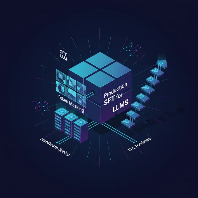

To fine-tune an LLM, load a base transformer checkpoint, freeze base model parameters using Parameter-Efficient Fine-Tuning (PEFT/LoRA) or 4-bit NormalFloat quantization (QLoRA), format instruction-response pairs into loss-masked token sequences, and compute cross-entropy gradients over the response tokens using Hugging Face TRL and FlashAttention-2. This process shifts model behavior, tone, and deterministic output formatting without retraining foundational parameters from scratch.
Most production engineering initiatives fail at the transition between generic prompt engineering and custom model training. Teams frequently run into out-of-memory (OOM) GPU crashes, catastrophic forgetting on out-of-domain benchmarks, or noisy training runs driven by corrupted instruction loss masking. Fine-tuning is not a mechanism for injecting dynamic factual knowledge, it is an optimization strategy for teaching specialized syntax, structured schema compliance, domain-specific tone, and low-latency task execution.
This architectural guide steps through the mathematical foundations of parameter adaptation, presents concrete VRAM formulas for hardware provisioning, and walks through a complete, production-grade PyTorch, TRL, and PEFT pipeline for modern transformer architectures in 2026.
Mechanics and Architecture: How LLM Fine-Tuning Works
Understanding what is fine tuning in the context of llms requires analyzing the transition from self-supervised pretraining to downstream task alignment. Foundation models undergo self-supervised pretraining across massive text corpora, optimizing standard causal language modeling objectives. The model minimizes cross-entropy loss by predicting the next token $x_t$ given an autoregressive context window of prior tokens:
$$\mathcal{L}_{\text{pretrain}}(\theta) = – \sum_{t=1}^{T} \log P_\theta(x_t \mid x_1, x_2, \dots, x_{t-1})$$
While this phase builds general linguistic capabilities and world knowledge, the raw base model acts as an open-ended probability distribution over text continuations rather than an instruction-following assistant. Fine tuning adapts this base checkpoint to specific functional behaviors by restricting the loss calculation to defined target tokens.
Key Architectural Rule: Modern supervised fine-tuning masks out the prompt tokens from the backward pass. Cross-entropy loss is computed strictly on response tokens, preventing the model from spending gradient capacity memorizing user prompts or system instructions.
So, how does llm fine tuning work beneath the surface? Supervised Fine-Tuning (SFT) adjusts the model weights $\theta$ toward a conditional distribution $P(Y \mid X)$, where $X$ represents an input instruction and $Y$ represents the desired completion:
$$\mathcal{L}_{\text{SFT}}(\theta) = – \sum_{i=1}^{|Y|} \log P_\theta(y_i \mid X, y_1, \dots, y_{i-1})$$
+--------------------------------------------------------------------------+
| Supervised Fine-Tuning Gradient Pipeline |
+--------------------------------------------------------------------------+
 [System Prompt + User Query (X)] --> [Response Tokens (Y)]
 | |
 Tokens: [ t1, t2, t3 ] Tokens: [ t4, t5, t6 ]
 Labels: [ -100, -100, -100 ] Labels: [ t4, t5, t6 ]
 | |
 (Masked Out) (Loss Calculated via AdamW)
 v v
 Zero Gradient Impact Weight Gradient Update: \Delta W
+--------------------------------------------------------------------------+
Executing finetuning large language models follows a systematic sequence of transformer state modifications:
- Representation Initialization: The base model loads pretrained weights into GPU memory, establishing fixed positional and attention projection spaces.
- Targeted Attention Projections: Instruction datasets route through self-attention layers ($W_q, W_k, W_v, W_o$) and feed-forward networks ($W_{\text{gate}}, W_{\text{up}}, W_{\text{down}}$).
- Loss Masking Application: Tokenizer components replace prompt label IDs with
-100, signaling the PyTorchCrossEntropyLossfunction to ignore them during backpropagation. - Gradient Computation and Backpropagation: Gradients flow through the computational graph, updating parameters or injected low-rank matrices via optimizer algorithms like AdamW or decoupled 8-bit variants.
- Distributional Shift: Through successive training epochs, probability mass redistributes to favor the stylistic, linguistic, and structural norms defined in the target training set.
Executing fine tuning models under this approach bridges the performance gap between unwieldy general-purpose base weights and deterministic operational agents. By constraining the gradient path, fine tuning llm checkpoints delivers tight schema outputs and high-throughput execution profiles.
Taxonomy of Model Fine-Tuning Techniques: Full Parameter vs. LoRA and QLoRA
When selecting model fine tuning techniques, machine learning engineers must weigh computational trade-offs, catastrophic forgetting risks, and inference deployment architectures. The three dominant llm fine tuning methods deployed in production environments are Full Fine-Tuning, Low-Rank Adaptation (LoRA), and Quantized Low-Rank Adaptation (QLoRA).
Full Parameter Fine-Tuning
Full fine tuning updates 100% of the parameters within the neural network. In a full finetuning run on a 70B parameter model, all 70 billion parameters receive gradient calculations and optimizer updates. While this offers maximum plasticity for massive domain shifts (such as learning a new natural language or compiling specialized programming languages), it introduces immense operational costs. Storing optimizer states, gradients, and model copies requires distributed GPU clusters running DeepSpeed ZeRO-3 or PyTorch Fully Sharded Data Parallel (FSDP). It also increases the risk of catastrophic forgetting, where the model degrades in broad reasoning and mathematical capabilities as it over-indexes on downstream data.
Low-Rank Adaptation (LoRA)
LoRA freezes the base model weights $W_0 \in \mathbb{R}^{d \times k}$ and injects trainable rank decomposition matrices into the transformer layers. The forward pass is modified by adding a parallel residual path:
$$h = W_0 x + \Delta W x = W_0 x + \frac{\alpha}{r} (B \cdot A) x$$
Here, $B \in \mathbb{R}^{d \times r}$ and $A \in \mathbb{R}^{r \times k}$, with the rank $r \ll \min(d, k)$. Typically, rank $r$ is chosen between 8 and 64, while $\alpha$ acts as a constant scaling factor. Matrix $A$ initializes from a random Gaussian distribution, while matrix $B$ initializes to zero, ensuring $\Delta W = 0$ at the start of training. LoRA typically trains less than 1% of the total network parameters, drastically cutting optimizer memory requirements.
Quantized Low-Rank Adaptation (QLoRA)
QLoRA builds upon LoRA by quantizing the frozen base model down to 4-bit NormalFloat (NF4), a mathematically optimal quantile distribution for normally distributed neural network weights. QLoRA introduces three primary optimizations:
- 4-bit NormalFloat (NF4): Quantizes FP16 weights to 4 bits while preserving theoretical information entropy.
- Double Quantization (DQ): Quantizes the quantization constants themselves, saving roughly 0.37 bits per parameter (approximately 3 GB on a 70B parameter checkpoint).
- Paged Optimizers: Leverages CUDA unified memory to dynamically page optimizer states between GPU VRAM and CPU system RAM during memory spikes, preventing OOM aborts.
Selection Rule: For enterprise classification, structured JSON extraction, and task-specific alignment, QLoRA and LoRA achieve parity with full fine-tuning while reducing VRAM footprints by 60% to 75%.
The table below provides a concrete engineering breakdown across the primary fine tuning ai models paradigms:
| Metric / Dimension | Full Parameter Fine-Tuning | LoRA (16-bit Base) | QLoRA (4-bit NF4 Base) |
|---|---|---|---|
| Base Weight Precision | FP16 / BF16 (16-bit) | FP16 / BF16 (16-bit) | NF4 / FP4 (4-bit) |
| Trainable Parameters | 100% | 0.1% to 1.5% | 0.1% to 1.5% |
| Optimizer Memory Footprint | High (~8x base weight size) | Minimal (tracks adapter only) | Minimal (tracks adapter only) |
| Typical 8B GPU Requirement | 4x to 8x A100 (80GB) via FSDP | 1x A100 (40GB/80GB) | 1x RTX 4090 / A5000 (24GB) |
| Typical 70B GPU Requirement | 32x to 64x H100 (80GB) via ZeRO-3 | 4x to 8x A100 (80GB) | 2x A100 (80GB) or 4x RTX 4090 |
| Throughput (Tokens/Sec/GPU) | High (baseline) | Moderate to High (~90% baseline) | Lower (~65-75% due to dequant) |
| Catastrophic Forgetting Risk | High | Low | Low |
| Deployment Flexibility | Single monolithic checkpoint | Modular adapter switching | Modular adapter switching |
Evaluating these llm fine tuning techniques demonstrates that unless deep vocabulary shifts or substantial foundational domain transformations are required, parameter-efficient fine tuning methods offer the most reliable balance of speed, cost, and task performance.
Hardware Sizing and VRAM Math for Fine-Tuning Training
Sizing GPU infrastructure for fine tuning training requires an understanding of where memory allocations go. Running out of memory during a training run halts processing instantly, wasting compute budgets. VRAM allocation during an active training loop is dictated by four distinct components:
$$\text{VRAM}_{\text{Total}} = M_{\text{weights}} + M_{\text{gradients}} + M_{\text{optimizer}} + M_{\text{activations}}$$
Deconstructing the Memory Components
- Model Weights ($M_{\text{weights}}$): The precision used to store model parameters determines this footprint. At 16-bit (FP16 or BF16), each parameter occupies 2 bytes. At 8-bit precision, each takes 1 byte. At 4-bit precision (NF4), each takes 0.5 bytes.
- Gradients ($M_{\text{gradients}}$): Gradients correspond directly to trainable parameters. Full fine-tuning stores gradients for every parameter at 16-bit precision (2 bytes per parameter). LoRA and QLoRA only calculate and store gradients for adapter weights, reducing this term to negligible sizes (often under 200 MB).
- Optimizer States ($M_{\text{optimizer}}$): Standard AdamW maintains two distinct dynamic moving states for every trainable parameter: the first momentum ($m_t$) and the second uncentered variance ($v_t$), both tracked in FP32 (4 bytes each) to preserve numerical stability. In addition, an FP32 master copy of the weights (4 bytes) is maintained, totaling 12 to 16 bytes per trainable parameter. Decoupled 8-bit optimizers (such as
bitsandbytes.optim.AdamW8bit) compress this overhead down to 2 to 4 bytes per parameter. - Activations ($M_{\text{activations}}$): Storing intermediate forward-pass tensor states for backward pass derivation scales linearly with batch size, sequence length, and transformer layer depth. Using FlashAttention-2 alongside activation checkpointing (gradient checkpointing) drops activation overhead from quadratic $O(N^2)$ to sub-linear, trading a ~20% compute overhead for dramatic memory reductions.
To evaluate your targets before executing a run to fine tune llm model checkpoints, run this bare-metal sizing calculation in Python:
def calculate_vram_requirements(
 params_in_billions: float,
 precision_bits: int,
 is_lora: bool = True,
 trainable_ratio: float = 0.01,
 batch_size: int = 4,
 seq_length: int = 4096,
 use_gradient_checkpointing: bool = True
) -> dict:
 # 1. Base model weights
 bytes_per_param = precision_bits / 8.0
 weight_gb = (params_in_billions * 1e9 * bytes_per_param) / (1024**3)

 # 2. Trainable parameters for gradients and optimizer states
 if is_lora:
 trainable_params = params_in_billions * 1e9 * trainable_ratio
 else:
 trainable_params = params_in_billions * 1e9

 # Gradients stored in FP16/BF16 (2 bytes)
 grad_gb = (trainable_params * 2.0) / (1024**3)

 # AdamW optimizer states (12 to 16 bytes per trainable param in FP32)
 opt_gb = (trainable_params * 12.0) / (1024**3)

 # 3. Activations approximation with FlashAttention-2 and Grad Checkpointing
 if use_gradient_checkpointing:
 # Highly reduced footprint: proportional to a few layer activations
 activation_gb = (batch_size * seq_length * 16 * 1024) / (1024**3)
 else:
 # Uncheckpointed activations scale aggressively with layers
 activation_gb = (batch_size * seq_length * 128 * 1024) / (1024**3)

 total_vram_gb = weight_gb + grad_gb + opt_gb + activation_gb
 # 20% margin for CUDA context, fragmentation, and runtime overhead
 recommended_gpu_vram = total_vram_gb * 1.20

 return {
 "Base Weights (GB)": round(weight_gb, 2),
 "Gradients (GB)": round(grad_gb, 2),
 "Optimizer States (GB)": round(opt_gb, 2),
 "Estimated Activations (GB)": round(activation_gb, 2),
 "Minimum Net VRAM (GB)": round(total_vram_gb, 2),
 "Recommended GPU Target (GB)": round(recommended_gpu_vram, 2)
 }

# Example calculation: 8B Parameter LLM via QLoRA (4-bit)
print(calculate_vram_requirements(8.0, precision_bits=4, is_lora=True))
The following hardware reference outlines production sizing expectations across diverse parameter tiers and training setups:
| Model Parameters | Training Strategy | Precision | Min Net VRAM | Recommended GPU Setup |
|---|---|---|---|---|
| 8B (e.g. Llama-3-8B) | Full Fine-Tuning | BF16 | ~120 GB | 2x A100 / H100 (80GB) via FSDP |
| 8B | LoRA (r=16, all modules) | BF16 | ~22 GB | 1x A100 (40GB) or RTX 6000 Ada |
| 8B | QLoRA (r=16, all modules) | NF4 | ~11 GB | 1x RTX 4090 / RTX 3090 (24GB) |
| 14B (e.g. Qwen-2.5-14B) | Full Fine-Tuning | BF16 | ~210 GB | 4x A100 / H100 (80GB) via FSDP |
| 14B | QLoRA (r=16, all modules) | NF4 | ~18 GB | 1x RTX 4090 / A5000 (24GB) |
| 70B (e.g. Llama-3.3-70B) | Full Fine-Tuning | BF16 | ~1050 GB | 16x H100 (80GB) via ZeRO-3 |
| 70B | LoRA (r=16, all modules) | BF16 | ~165 GB | 4x A100 / H100 (80GB) |
| 70B | QLoRA (r=16, all modules) | NF4 | ~52 GB | 1x H100 (80GB) or 2x A100 (80GB) |
Correct hardware sizing ensures stable convergence while preserving your hardware spend, matching appropriate fine tuning parameters to target infrastructure limits to maintain peak fine tune performance.
Dataset Curation and Formatting Pipelines
Data hygiene dictates the outcome of any model training initiative. Low-quality datasets yield low-quality generations regardless of how carefully you tune hyperparameters. When executing fine tuning large language models, your dataset must be cleaned, de-duplicated, formatted into structured schemas, and tokenized with correct label masking.
Format Selection: Alpaca vs. ShareGPT
Two primary schema designs dominate instruction tuning pipelines:
- Alpaca Format: Suited for single-turn task execution, input-output mappings, and straightforward extraction pipelines. It contains discrete fields for
instruction,input, andoutput. - ShareGPT Format: Suited for conversational threads, stateful multi-turn interactions, and context-dependent workflows. It organizes data as a sequential list of objects containing
from(system, human, or gpt) andvaluefields.
import json
from datasets import Dataset

# Canonical modern chat template format (OpenAI/Hugging Face ChatML style)
raw_samples = [
 {
 "messages": [
 {"role": "system", "content": "You are a strict data validation engine. Output valid JSON only."},
 {"role": "user", "content": "Parse entity: AcmeCorp registered in Delaware on 2021-05-12."},
 {"role": "assistant", "content": "{\"company\": \"AcmeCorp\", \"state\": \"Delaware\", \"incorporated\": \"2021-05-12\"}"}
 ]
 }
]

def apply_chat_template(batch, tokenizer):
 formatted_texts = []
 for conversation in batch["messages"]:
 # Formats into canonical template tags: <|im_start|>system..<|im_end|>
 text = tokenizer.apply_chat_template(
 conversation,
 tokenize=False,
 add_generation_prompt=False
 )
 formatted_texts.append(text)
 return {"text": formatted_texts}

# Convert to Hugging Face dataset format
hf_dataset = Dataset.from_list(raw_samples)
Preparing clean data for the fine tuning process requires validating each transformation step before initiating compute jobs:
- Deduplication: Filter raw inputs using MinHash LSH to purge identical and near-duplicate instructional pairs, preventing over-indexation and mode collapse.
- Contamination Filtering: Scrub your fine-tuning corpus of any evaluation prompts or benchmark validation data (such as HumanEval, GSM8k, or internal holdout tests) to eliminate false metric inflation.
- Length Truncation Checks: Run empirical token count analyses over all entries. Choose maximum sequence lengths that capture 95% to 99% of sample token lengths without wasting padding memory.
- Chat Template Alignment: Verify that the tokenizer chat template matches the base model pretraining specification (e.g. Llama-3 format vs. ChatML vs. Mistral token templates).
- Explicit Label Masking: Confirm that the loss calculation step replaces prompt and system token IDs with
-100, restricting backpropagation strictly to downstream assistant response targets.
Adhering to this pipeline prevents training run contamination and ensures consistent gradient updates throughout finetuning llms.
Step-by-Step LLM Fine-Tuning Tutorial with PyTorch, TRL, and PEFT
This section provides a production-grade implementation of how to fine tune an llm using Hugging Face transformers, peft, bitsandbytes, and trl. This script demonstrates how to fine tune a large language model using 4-bit QLoRA, integrating FlashAttention-2 and gradient checkpointing for optimal memory efficiency.
- Environment Preparation: Initialize your target Python virtual environment and ensure you have installed modern CUDA-compatible libraries (
torch>=2.4.0,transformers>=4.48.0,peft>=0.14.0,trl>=0.14.0, andbitsandbytes>=0.45.0). - Quantization Configuration: Construct a
BitsAndBytesConfigobject enforcing 4-bit NormalFloat precision with double quantization enabled. - Base Model Instantiation: Load the base transformer using low-CPU memory initialization and
bfloat16compute precision. - LoRA Adapter Parameterization: Instantiate a
LoraConfigtargeting all linear projection layers (q_proj,k_proj,v_proj,o_proj,gate_proj,up_proj,down_proj). - SFTTrainer Execution: Pass the configured components, tokenized dataset, and training arguments to the
SFTTrainerto run the training loop.
Here is the complete, self-contained llm fine tuning tutorial code block:
import torch
from datasets import load_dataset
from transformers import (
 AutoModelForCausalLM,
 AutoTokenizer,
 BitsAndBytesConfig,
 TrainingArguments
)
from peft import LoraConfig, get_peft_model, prepare_model_for_kbit_training
from trl import SFTTrainer

def run_finetuning_pipeline():
 model_id = "meta-llama/Llama-3.1-8B-Instruct"

 # 1. 4-bit Quantization Configuration for QLoRA
 bnb_config = BitsAndBytesConfig(
 load_in_4bit=True,
 bnb_4bit_quant_type="nf4",
 bnb_4bit_compute_dtype=torch.bfloat16,
 bnb_4bit_use_double_quant=True
 )

 # 2. Tokenizer Setup
 tokenizer = AutoTokenizer.from_pretrained(model_id, use_fast=True)
 if tokenizer.pad_token is None:
 tokenizer.pad_token = tokenizer.eos_token
 tokenizer.padding_side = "right" # Prevents issues in causal decoder attention

 # 3. Model Loading with FlashAttention-2
 model = AutoModelForCausalLM.from_pretrained(
 model_id,
 quantization_config=bnb_config,
 device_map="auto",
 attn_implementation="flash_attention_2",
 torch_dtype=torch.bfloat16
 )

 # Prepare model for stable k-bit adapter training
 model = prepare_model_for_kbit_training(model, use_gradient_checkpointing=True)

 # 4. LoRA Adapter Hyperparameters Configuration
 peft_config = LoraConfig(
 r=16,
 lora_alpha=32,
 target_modules=[
 "q_proj", "k_proj", "v_proj", "o_proj",
 "gate_proj", "up_proj", "down_proj"
 ],
 lora_dropout=0.05,
 bias="none",
 task_type="CAUSAL_LM"
 )

 # 5. Training Hyperparameters Configuration
 training_args = TrainingArguments(
 output_dir="./llama3-finetuned-output",
 per_device_train_batch_size=2,
 gradient_accumulation_steps=8, # Effective batch size = 16
 learning_rate=2e-4,
 lr_scheduler_type="cosine",
 warmup_ratio=0.03,
 num_train_epochs=3,
 logging_steps=10,
 save_strategy="steps",
 save_steps=100,
 save_total_limit=2,
 bf16=True,
 fp16=False,
 optim="paged_adamw_8bit", # Saves VRAM by offloading optimizer spikes
 max_grad_norm=0.3, # Prevents gradient explosion
 logging_first_step=True,
 report_to="none"
 )

 # 6. Mock dataset for illustration
 train_dataset = load_dataset("philschmid/dolly-15k-curated-en", split="train[:1000]")

 # 7. SFTTrainer Execution
 trainer = SFTTrainer(
 model=model,
 train_dataset=train_dataset,
 peft_config=peft_config,
 dataset_text_field="context",
 max_seq_length=2048,
 tokenizer=tokenizer,
 args=training_args
 )

 print("Starting fine-tuning run..")
 trainer.train()

 # 8. Save the final adapter weights
 trainer.model.save_pretrained("./llama3-final-adapter")
 tokenizer.save_pretrained("./llama3-final-adapter")
 print("Adapter successfully exported to disk.")

if __name__ == "__main__":
 run_finetuning_pipeline()
This llm fine tuning example consolidates best practices into a reproducible pipeline. By pairing paged_adamw_8bit with FlashAttention-2, gradient checkpointing, and target module adapter coverage, this configuration enables reliable execution on consumer hardware while preserving the numerical stability needed to effectively finetune llm models for production environments.
Post-Training Evaluation, Adapter Merging, and Production Deployment
Completing a training loop is only half the engineering lifecycle. Once adapter weights finish training, machine learning engineers must evaluate model drift, merge the adapter parameters back into base precision weights, and deploy the artifact to a high-throughput inference engine.
The 5-Tier Evaluation Strategy
Avoid relying solely on raw validation loss, which measures predictive perplexity rather than task compliance. Deploy a comprehensive evaluation framework instead:
- Automated Loss and Perplexity: Track validation loss curves to ensure steady convergence without overfitting.
- Benchmark Drift Testing: Run baseline capabilities benchmarks (MMLU, GSM8k) to quantify any drop in broad reasoning skills.
- Deterministic Output Parsing: For structured output tasks, measure schema parse rates (such as JSON validation) over held-out test splits.
- LLM-as-a-Judge Evaluation: Use high-capability evaluator models (such as GPT-4o or Claude 3.5 Sonnet) to score completions against ground-truth references based on clear grading criteria.
- Human Spot-Checking: Manually audit low-scoring and edge-case samples to identify subtle failures, hallucinations, or behavioral edge cases.
Adapter Merging and Serialization
Deploying standalone adapters atop quantized base weights in production introduces inference latency overhead from parallel forward paths. The optimal strategy is merging the adapter matrix $\Delta W = \frac{\alpha}{r} (B \cdot A)$ directly into the base weights $W_0$, serializing an unquantized 16-bit model for production inference:
import torch
from peft import PeftModel
from transformers import AutoModelForCausalLM, AutoTokenizer

def merge_and_export_model():
 base_model_path = "meta-llama/Llama-3.1-8B-Instruct"
 adapter_path = "./llama3-final-adapter"
 export_destination = "./llama3-merged-production"

 print("Loading unquantized base model in FP16/BF16..")
 # Note: Adapter merging requires an unquantized base checkpoint
 base_model = AutoModelForCausalLM.from_pretrained(
 base_model_path,
 return_dict=True,
 torch_dtype=torch.bfloat16,
 device_map="cpu" # Avoids consuming GPU memory during conversion
 )

 tokenizer = AutoTokenizer.from_pretrained(base_model_path)

 print("Loading trained PEFT adapter..")
 peft_model = PeftModel.from_pretrained(base_model, adapter_path)

 print("Merging adapter weights into base model layers..")
 # Merges W_new = W_0 + (alpha/r)*(B x A) directly into base weights
 merged_model = peft_model.merge_and_unload()

 print(f"Writing full checkpoint to: {export_destination}")
 merged_model.save_pretrained(export_destination, safe_serialization=True)
 tokenizer.save_pretrained(export_destination)
 print("Model merge complete. Checkpoint is ready for deployment.")

if __name__ == "__main__":
 merge_and_export_model()
High-Throughput Serving via vLLM
Once your merged checkpoint is saved to disk, serve it using high-performance inference frameworks like vLLM. vLLM implements PagedAttention to eliminate memory fragmentation in KV-cache storage, supporting high concurrency and low latency.
Launch the serving instance from the terminal:
# Serve the merged checkpoint across 1x GPU with PagedAttention and an OpenAI-compatible endpoint
vllm serve./llama3-merged-production \
 --host 0.0.0.0 \
 --port 8000 \
 --tensor-parallel-size 1 \
 --dtype bfloat16 \
 --max-model-len 4096 \
 --gpu-memory-utilization 0.90
Following this release process allows you to fine tune llms with low training costs while serving responsive, deterministic inference endpoints in production. This bridges the path from initial dataset assembly to a reliable, scalable deployment when finetuning large language models.
Frequently Asked Questions
LLMs can be fine tuned using which technique for resource-constrained environments?
LLMs can be fine tuned in resource-constrained environments using Parameter-Efficient Fine-Tuning (PEFT), primarily QLoRA. QLoRA quantizes base weights to 4-bit precision while updating low-rank adapter matrices in 16-bit, cutting VRAM demands by over 65% while matching full fine-tuning performance.
What is the primary difference between fine-tuning and prompt engineering?
Prompt engineering adjusts in-context inference tokens without modifying neural network parameters. Fine-tuning adjusts the underlying transformer layer weights or adapter matrices through backpropagation, baking domain-specific style, tone, and deterministic formatting directly into the model architecture.
When should you choose fine-tuning over Retrieval-Augmented Generation (RAG)?
Choose fine-tuning when the objective is mastering specific syntax, specialized terminology, structured schemas (such as JSON extraction), or stylistic tone. Choose RAG when models require dynamic, up-to-date factual retrieval from external databases with low tolerance for hallucination.
How do you prevent catastrophic forgetting during supervised fine-tuning?
Prevent catastrophic forgetting by using parameter-efficient adapters like LoRA rather than full parameter updates, adding a 5-10% replay buffer of general domain pretraining data, enforcing low learning rates (1e-5 to 2e-4), and monitoring validation loss on broad benchmarks like MMLU.
What are critical engineering considerations for fine tuning llms?
When implementing fine tuning llms, prioritize deterministic execution, rigorous error handling, observability metrics, and strict security isolation to maintain production reliability and eliminate latency bottlenecks.
What are critical engineering considerations for fine tuning llm models?
When implementing fine tuning llm models, prioritize deterministic execution, rigorous error handling, observability metrics, and strict security isolation to maintain production reliability and eliminate latency bottlenecks.
What are critical engineering considerations for finetune ai?
When implementing finetune ai, prioritize deterministic execution, rigorous error handling, observability metrics, and strict security isolation to maintain production reliability and eliminate latency bottlenecks.
Mastering modern model adaptation requires moving past abstract concepts to build structured, reproducible training pipelines. Using Parameter-Efficient Fine-Tuning frameworks like LoRA and QLoRA, engineering teams can adapt foundation models to strict formatting guidelines, specialized business domain vocabularies, and optimized latency requirements, without needing large-scale supercomputer hardware.
As you run fine-tuning jobs in production, maintain rigorous data hygiene, enforce strict instruction loss masking, calculate memory requirements accurately before launching clusters, and evaluate adapted weights across task accuracy and general capabilities. With toolsets like Hugging Face TRL, PEFT, and vLLM, small engineering teams can reliably build, validate, and serve custom models built for specific production workloads.