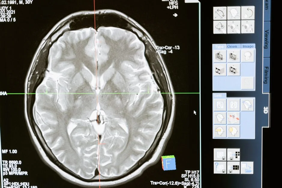

Image segmentation is a computer vision technique that partitions a digital image into multiple segments or sets of pixels, often to identify and locate objects, boundaries, and specific regions within the image. This process assigns a label to every pixel in an image such that pixels with the same label share certain characteristics, enabling precise object extraction and analysis. It is a foundational task for advanced applications such as autonomous driving, medical imaging, and augmented reality, providing granular understanding beyond simple object detection.
The current adoption of image segmentation spans critical industries, driven by advancements in deep learning. From enhancing diagnostic accuracy in healthcare by isolating tumors and organs to enabling precise robotic manipulation in manufacturing and powering sophisticated visual effects in entertainment, segmentation has become an indispensable tool. Its integration into complex systems necessitates robust architectural patterns and careful consideration of computational resources, data management, and model deployment strategies.
Core Concepts and Taxonomy of Image Segmentation
Image segmentation fundamentally involves dividing an image into constituent parts or objects. This process is distinct from object detection, which merely draws bounding boxes around objects, and image classification, which assigns a single label to an entire image. Segmentation operates at a pixel level, providing a much finer-grained understanding of an image’s content. There are three primary types of image segmentation, each serving different analytical purposes and requiring distinct algorithmic approaches.
Semantic Segmentation: Pixel-Level Classification
Semantic segmentation aims to classify each pixel in an image into a predefined set of categories, such as ‘person,’ ‘car,’ or ‘road.’ All pixels belonging to the same semantic class are assigned the same label, regardless of whether they represent distinct instances of that class. For example, in an image containing multiple cars, semantic segmentation would label all car pixels identically, treating them as one collective ‘car’ class. The output is typically a segmentation map where each pixel’s value corresponds to its assigned class.
This approach is particularly useful in applications where the specific instance of an object is less important than its general presence and spatial distribution. Examples include:
- Autonomous Driving: Identifying navigable roads, sidewalks, and general obstacles like vehicles and pedestrians. The system needs to know ‘where the road is’ rather than ‘which specific car is which.’
- Medical Imaging: Delineating tissue types, organs, or abnormalities in scans. For instance, segmenting ‘tumor’ regions from ‘healthy tissue’ without needing to differentiate between individual tumor cells.
- Geospatial Analysis: Classifying land cover types such as forests, water bodies, and urban areas from satellite imagery.
Architecturally, semantic segmentation models typically employ an encoder-decoder structure. The encoder progressively downsamples the input image, capturing high-level semantic features, while the decoder upsamples these features to reconstruct a segmentation map at the original image resolution. Skip connections are often used to preserve fine-grained spatial information lost during downsampling, leading to more accurate boundary predictions.
Instance Segmentation: Object-Specific Delineation
Instance segmentation takes semantic segmentation a step further by identifying and segmenting individual instances of objects. While semantic segmentation labels all pixels belonging to the ‘car’ class uniformly, instance segmentation would differentiate between ‘car 1,’ ‘car 2,’ and ‘car 3,’ providing a unique mask for each. This requires both accurate pixel classification and the ability to distinguish between separate objects of the same class.
This form of segmentation is critical when an application needs to interact with or analyze individual objects. Common applications include:
- Robotics: Enabling robots to grasp specific objects by providing precise masks of each item in a cluttered environment.
- Retail Analytics: Counting individual customers or products on shelves, analyzing their movements, or identifying specific items for inventory management.
- Video Surveillance: Tracking individual people or vehicles over time, which is essential for security and traffic analysis.
Popular models for instance segmentation, such as Mask R-CNN, often combine object detection with semantic segmentation. They first detect object bounding boxes and then, for each detected box, predict a pixel-level mask. This dual-task approach adds complexity but yields significantly richer information about the scene. Implementing such models in production requires careful consideration of computational resources, particularly GPU memory and processing power, as they are inherently more resource-intensive than semantic segmentation models.
Panoptic Segmentation: Unifying Semantic and Instance Views
Panoptic segmentation is a relatively newer task that unifies semantic and instance segmentation. It aims to assign a semantic label and an instance ID to every pixel in an image. This means that ‘stuff’ classes (e.g., road, sky, grass), which are typically amorphous and do not have distinct instances, are semantically segmented, while ‘thing’ classes (e.g., person, car, animal), which are countable objects, are instance segmented. Every pixel in the image is assigned exactly one semantic label and, if applicable, one instance ID.
The goal of panoptic segmentation is to provide a complete and unambiguous scene understanding. This comprehensive output is highly valuable for applications that require both a general understanding of the environment and precise interaction with individual objects.
- Advanced Autonomous Systems: A self-driving car needs to know not only where the road is (semantic) but also the exact boundaries and identities of individual pedestrians and other vehicles (instance) to make safe navigation decisions.
- Augmented Reality: Accurately placing virtual objects into a real-world scene requires a detailed understanding of both background surfaces and foreground objects to ensure realistic occlusion and interaction.
- Human-Computer Interaction: Understanding complex user environments for advanced gesture recognition or contextual computing.
Developing panoptic segmentation models often involves multi-task learning architectures that simultaneously predict semantic masks and instance masks, then fuse them into a consistent panoptic map. This integration requires sophisticated model design and robust post-processing logic to resolve conflicts and ensure pixel uniqueness across semantic and instance predictions. The complexity of these models translates directly to increased demands on training data, computational resources, and careful system design for deployment.
Key Algorithms and Deep Learning Models for Segmentation
The field of image segmentation has been revolutionized by deep learning, moving beyond traditional methods to achieve unprecedented accuracy and robustness. Modern segmentation relies heavily on convolutional neural networks (CNNs), which can learn hierarchical features from images. Understanding the architecture of these key models is crucial for effective implementation and optimization.
U-Net: Pioneering Biomedical Segmentation
The U-Net architecture, introduced in 2015, was specifically designed for biomedical image segmentation, excelling in scenarios with limited training data. Its distinctive ‘U’ shape consists of a contracting path (encoder) that captures context and an expansive path (decoder) that enables precise localization. Crucially, U-Net employs ‘skip connections’ that directly concatenate feature maps from the contracting path to the expansive path at corresponding resolution levels. This allows the decoder to recover fine-grained spatial information that might be lost during the downsampling process, leading to highly accurate boundary predictions.
The encoder part typically consists of repeated application of 3×3 convolutions, followed by a rectified linear unit (ReLU) and a 2×2 max pooling operation for downsampling. Each downsampling step halves the spatial dimensions while doubling the number of feature channels. The decoder mirrors this, using up-convolutions (transposed convolutions) to upsample feature maps, followed by 3×3 convolutions and ReLU activations. The skip connections ensure that high-resolution features from the encoder are available to the decoder, which is vital for precise localization.
import torchimport torch.nn as nnclass DoubleConv(nn.Module): """(convolution => BN => ReLU) * 2""" def __init__(self, in_channels, out_channels): super().__init__() self.double_conv = nn.Sequential( nn.Conv2d(in_channels, out_channels, kernel_size=3, padding=1), nn.BatchNorm2d(out_channels), nn.ReLU(inplace=True), nn.Conv2d(out_channels, out_channels, kernel_size=3, padding=1), nn.BatchNorm2d(out_channels), nn.ReLU(inplace=True) ) def forward(self, x): return self.double_conv(x)class Up(nn.Module): """Upscaling then double conv""" def __init__(self, in_channels, out_channels, bilinear=True): super().__init__() if bilinear: self.up = nn.Upsample(scale_factor=2, mode='bilinear', align_corners=True) self.conv = DoubleConv(in_channels, out_channels) else: self.up = nn.ConvTranspose2d(in_channels, in_channels // 2, kernel_size=2, stride=2) self.conv = DoubleConv(in_channels, out_channels) def forward(self, x1, x2): # x1 is upsampled, x2 is from encoder x1 = self.up(x1) # Pad x1 if necessary to match x2's size (common in U-Net implementations) diffY = x2.size()[2] - x1.size()[2] diffX = x2.size()[3] - x1.size()[3] x1 = nn.functional.pad(x1, [diffX // 2, diffX - diffX // 2, diffY // 2, diffY - diffY // 2]) x = torch.cat([x2, x1], dim=1) # Concatenate along channel dimension return self.conv(x)class UNet(nn.Module): def __init__(self, n_channels, n_classes, bilinear=True): super(UNet, self).__init__() self.n_channels = n_channels self.n_classes = n_classes self.bilinear = bilinear self.inc = DoubleConv(n_channels, 64) self.down1 = nn.MaxPool2d(2) self.conv1 = DoubleConv(64, 128) self.down2 = nn.MaxPool2d(2) self.conv2 = DoubleConv(128, 256) self.down3 = nn.MaxPool2d(2) self.conv3 = DoubleConv(256, 512) self.down4 = nn.MaxPool2d(2) self.conv4 = DoubleConv(512, 1024 // (2 if bilinear else 1)) self.up1 = Up(1024, 512 // (2 if bilinear else 1), bilinear) self.up2 = Up(512, 256 // (2 if bilinear else 1), bilinear) self.up3 = Up(256, 128 // (2 if bilinear else 1), bilinear) self.up4 = Up(128, 64, bilinear) self.outc = nn.Conv2d(64, n_classes, kernel_size=1) def forward(self, x): x1 = self.inc(x) x2 = self.conv1(self.down1(x1)) x3 = self.conv2(self.down2(x2)) x4 = self.conv3(self.down3(x3)) x5 = self.conv4(self.down4(x4)) x = self.up1(x5, x4) x = self.up2(x, x3) x = self.up3(x, x2) x = self.up4(x, x1) logits = self.outc(x) return logits# Example Usage: # model = UNet(n_channels=3, n_classes=2) # 3 input channels (RGB), 2 output classes (e.g., background, foreground) # input_tensor = torch.randn(1, 3, 256, 256) # Batch size 1, 3 channels, 256x256 image # output = model(input_tensor) # print(output.shape) # Expected: torch.Size([1, 2, 256, 256])U-Net’s efficiency and ability to generalize from smaller datasets make it a strong candidate for applications where data annotation is costly or limited. Its architecture also forms the basis for many subsequent segmentation models.
Mask R-CNN: Instance Segmentation Powerhouse
Mask R-CNN is a seminal work in instance segmentation, extending the Faster R-CNN object detection framework. It performs both object detection (bounding box regression and classification) and pixel-level segmentation for each detected object instance. This model works in two stages: first, a Region Proposal Network (RPN) proposes candidate object bounding boxes. Second, for each proposal, a RoIAlign (Region of Interest Align) layer precisely extracts features, which are then fed into three parallel branches: one for classification, one for bounding box regression, and a new branch for predicting a binary mask for each class.
The RoIAlign layer is a critical improvement over its predecessor, RoIPool, as it uses bilinear interpolation to accurately align feature maps with the original image coordinates, preserving spatial information vital for precise mask generation. This meticulous alignment avoids quantization errors, leading to significantly better mask quality.
The Mask R-CNN architecture typically uses a deep backbone network, such as ResNet or ResNeXt, pre-trained on ImageNet for feature extraction. The RPN and subsequent heads are then built on top of these features. The multi-task loss function combines the classification loss, bounding box regression loss, and mask prediction loss, allowing the network to learn all three tasks simultaneously.
While powerful, Mask R-CNN is computationally more intensive than U-Net due to its multi-stage nature and the complexity of predicting masks for multiple instances. Deployment in real-time systems often requires powerful GPU acceleration and careful optimization, potentially through techniques like model pruning or quantization. For backend systems integrating with such a model, an asynchronous processing pipeline, possibly leveraging a Java Queue API or similar message broker, would be essential to handle the inference load without blocking the main application thread.
DeepLab Family: Advancing Semantic Segmentation
The DeepLab series of models (DeepLabv1, v2, v3, v3+) has significantly pushed the boundaries of semantic segmentation. Key innovations across the DeepLab family include:
- Atrous Convolution (Dilated Convolution): This technique allows filters to have a wider field of view without increasing the number of parameters or losing resolution. It effectively captures multi-scale context by applying filters with holes, allowing them to sample features from a larger receptive field.
- Atrous Spatial Pyramid Pooling (ASPP): DeepLabv2 introduced ASPP, which applies atrous convolutions with different rates in parallel to capture context at multiple scales. This helps in segmenting objects of various sizes. DeepLabv3 refined this by incorporating batch normalization and image-level features.
- Encoder-Decoder Structure (DeepLabv3+): DeepLabv3+ combined the strengths of atrous convolution and ASPP with an encoder-decoder structure, similar to U-Net. The encoder extracts rich semantic information using atrous convolutions, while the decoder gradually recovers spatial information to produce sharp object boundaries. This hybrid approach allows for both robust feature extraction and precise localization.
DeepLab models, particularly DeepLabv3+, offer a strong balance between accuracy and computational efficiency for semantic segmentation tasks. Their ability to handle objects at multiple scales makes them highly effective in diverse environments. For production deployment, considerations include selecting an appropriate backbone network (e.g., ResNet, Xception), optimizing atrous rates, and potentially leveraging hardware accelerators. These models are often used in cloud-based inference services where computational resources can be scaled on demand.
Traditional Segmentation Methods (Briefly)
While deep learning dominates, it’s worth noting traditional methods still have niche applications or serve as foundational concepts:
- Thresholding: Simple methods like Otsu’s method divide an image into foreground and background based on pixel intensity. Effective for high-contrast images.
- Clustering-based Methods: K-means clustering can group pixels based on color or intensity similarity.
- Region-based Methods: Techniques like region growing or watershed algorithms group adjacent pixels with similar properties into regions. The watershed algorithm is particularly useful for separating touching objects.
- Edge-based Methods: Using edge detection (e.g., Canny, Sobel) to find object boundaries.
These traditional methods are generally faster but less robust to variations in lighting, texture, and object appearance compared to deep learning models. They may be suitable for simpler, highly constrained environments or as pre-processing steps.
Architectural Considerations for Production Segmentation Systems
Deploying image segmentation models into production requires more than just training an accurate model; it demands a robust, scalable, and maintainable system architecture. Backend engineers must consider data pipelines, inference scalability, latency requirements, and integration with existing services. A well-designed architecture ensures reliable performance, efficient resource utilization, and ease of maintenance.
Data Ingestion and Pre-processing Pipelines
The journey of an image through a segmentation system begins with data ingestion. Images can originate from various sources: user uploads, IoT devices, surveillance cameras, or internal databases. A robust ingestion pipeline must handle diverse formats, resolutions, and volumes. This often involves:
- Message Queues: Using systems like Kafka, RabbitMQ, or AWS SQS to decouple the ingestion process from downstream processing. This allows for asynchronous handling of image data, preventing bottlenecks and ensuring system resilience. For handling asynchronous tasks in a Laravel context, integrating with a message queue can be done via Laravel Queues, which abstracts away the underlying queue driver.
- Cloud Storage: Storing raw and processed images in scalable, highly available object storage services (e.g., Amazon S3, Google Cloud Storage). This provides durability and accessibility for further processing.
- Pre-processing Modules: Before inference, images often require normalization, resizing, color space conversion, and potentially augmentation. These steps should be encapsulated in reusable, efficient modules. A common pattern is to use serverless functions or dedicated microservices for these tasks, allowing for independent scaling.
# Example: A simplified Python function for image pre-processingimport cv2import numpy as npdef preprocess_image(image_bytes: bytes, target_size=(512, 512)) -> np.ndarray: """ Decodes image bytes, resizes, normalizes, and prepares for model inference. Args: image_bytes: Raw image data as bytes. target_size: Tuple (height, width) for resizing. Returns: Numpy array of the preprocessed image. Raises: ValueError: If image decoding fails. """ try: # Decode image from bytes nparr = np.frombuffer(image_bytes, np.uint8) img = cv2.imdecode(nparr, cv2.IMREAD_COLOR) if img is None: raise ValueError("Could not decode image from bytes.") # Resize image img_resized = cv2.resize(img, target_size, interpolation=cv2.INTER_AREA) # Normalize pixel values to [0, 1] and change channel order (e.g., BGR to RGB) img_normalized = img_resized.astype(np.float32) / 255.0 img_normalized = cv2.cvtColor(img_normalized, cv2.COLOR_BGR2RGB) # Add batch dimension (model expects [batch_size, height, width, channels] or [batch_size, channels, height, width]) # Assuming TensorFlow/Keras channel-last format for this example img_final = np.expand_dims(img_normalized, axis=0) return img_final except Exception as e: print(f"Error during image pre-processing: {e}") raise ValueError(f"Image pre-processing failed: {e}")# In a production system, this would be part of a microservice# or a dedicated processing worker that consumes from a message queue.Model Inference and Deployment Strategies
The core of the system is the inference service. Its design heavily depends on latency requirements and expected throughput.
- Synchronous APIs: For low-latency, real-time applications (e.g., AR, interactive UIs), a synchronous REST API endpoint might be exposed. This requires the inference service to be highly optimized and potentially utilize GPU-accelerated instances. Load balancers and auto-scaling groups are essential for handling variable traffic.
- Asynchronous Processing: For tasks that can tolerate higher latency (e.g., batch processing, background analysis), an asynchronous approach is often preferred. Clients upload images, receive a job ID, and poll for results or get notified via webhooks. This pattern is ideal for integrating with a Laravel HTTP Client managing external service calls. Message queues are central here, allowing inference workers to pull tasks as resources become available.
- Serverless Functions: For sporadic or bursty workloads, serverless platforms (AWS Lambda, Google Cloud Functions) can host inference logic. While convenient, cold start times and resource limits need careful consideration, especially for large models.
- Containerization (Docker) and Orchestration (Kubernetes): Packaging models and their dependencies into Docker containers ensures consistency across development, testing, and production environments. Kubernetes then provides robust orchestration for deploying, scaling, and managing these containers, offering high availability and fault tolerance. This aligns with modern practices for architecting production-grade deployments.
- Edge Deployment: For scenarios requiring extremely low latency or offline capabilities (e.g., embedded devices, drones), models can be optimized and deployed directly on edge hardware. This often involves model quantization, pruning, and specialized inference engines (e.g., TensorRT, OpenVINO).
Post-processing and Result Storage
After inference, the raw segmentation masks often require post-processing:
- Refinement: Applying morphological operations (erosion, dilation), connected component analysis, or conditional random fields (CRFs) to refine mask boundaries.
- Metadata Generation: Extracting statistics (e.g., object counts, areas, centroids) from the masks.
- Result Storage: Storing segmentation masks and associated metadata. Masks can be stored as binary images (PNG), run-length encoded (RLE) strings for efficiency, or polygon representations in databases. Metadata should be stored in a structured database (SQL or NoSQL) for easy querying and analysis.
Monitoring and Observability
A production system is incomplete without robust monitoring. Key metrics include:
- System Metrics: CPU/GPU utilization, memory usage, network I/O, disk space.
- Application Metrics: Request rates, latency (P50, P90, P99), error rates, queue lengths.
- Model Performance Metrics: Monitoring model accuracy on a subset of production data to detect model drift or performance degradation over time.
Logging, tracing, and alerting systems (e.g., Prometheus, Grafana, ELK Stack, Jaeger) are essential for quickly identifying and diagnosing issues. A proactive approach to monitoring helps maintain system health and model efficacy.
Data Management and Annotation Challenges
High-quality data is the lifeblood of deep learning models, and image segmentation is particularly data-hungry. The challenges in data management for segmentation revolve around acquisition, annotation, storage, and versioning. Addressing these challenges effectively is paramount for building robust and accurate models.
The Annotation Bottleneck
Image segmentation models require pixel-perfect ground truth masks for training. This means a human annotator must meticulously outline the boundaries of every object of interest in thousands, if not tens of thousands, of images. This process is:
- Time-Consuming: Delineating complex shapes pixel by pixel is incredibly laborious, especially for high-resolution images or numerous objects per image.
- Expensive: Due to the manual effort involved, annotation is a significant cost driver in any segmentation project.
- Error-Prone: Human annotators can introduce inconsistencies or inaccuracies, especially when dealing with ambiguous boundaries or fatigue. Quality control mechanisms are therefore crucial.
- Expertise-Dependent: In specialized domains like medical imaging, annotation requires domain experts, further increasing cost and complexity.
To mitigate the annotation bottleneck, several strategies are employed:
- Active Learning: The model identifies images or regions where it is uncertain and requests human annotation only for those specific, high-value samples. This focuses human effort where it matters most.
- Semi-Supervised Learning: Leveraging a small amount of labeled data alongside a large amount of unlabeled data. Techniques like pseudo-labeling or consistency regularization can help models learn from unannotated examples.
- Weakly Supervised Learning: Training models with coarser labels, such as bounding boxes or image-level tags, and inferring pixel-level masks. While less precise than full supervision, it can drastically reduce annotation costs.
- Transfer Learning: Fine-tuning pre-trained models on smaller, domain-specific datasets. This reduces the need for massive domain-specific datasets from scratch.
- Automated Annotation Tools: Using AI-assisted tools that provide initial mask predictions for human annotators to refine, speeding up the process.
# Conceptual Python code for an active learning loop (simplified)from sklearn.ensemble import RandomForestClassifier # Example uncertainty modelfrom sklearn.model_selection import train_test_splitimport numpy as np# Assume we have a pool of unlabeled_data and a small labeled_data_X, labeled_data_y# labeled_data_X: features (e.g., image embeddings), labeled_data_y: ground truth masks# In a real scenario, 'features' would be derived from an initial segmentation model's outputdef calculate_uncertainty(model, X_unlabeled): # A simple uncertainty measure: entropy of predicted probabilities probabilities = model.predict_proba(X_unlabeled) entropy = -np.sum(probabilities * np.log(probabilities + 1e-9), axis=1) return entropydef active_learning_iteration(model, labeled_X, labeled_y, unlabeled_X, num_to_annotate=10): # Train model on current labeled data model.fit(labeled_X, labeled_y) # Calculate uncertainty for unlabeled data uncertainties = calculate_uncertainty(model, unlabeled_X) # Select the most uncertain samples most_uncertain_indices = np.argsort(uncertainties)[-num_to_annotate:] # Simulate human annotation for these samples (in reality, this is a manual step) newly_labeled_X = unlabeled_X[most_uncertain_indices] newly_labeled_y = simulate_human_annotation(newly_labeled_X) # Placeholder for actual human work # Update labeled and unlabeled sets labeled_X = np.vstack([labeled_X, newly_labeled_X]) labeled_y = np.vstack([labeled_y, newly_labeled_y]) # Or concatenate if y is a list unlabeled_X = np.delete(unlabeled_X, most_uncertain_indices, axis=0) return model, labeled_X, labeled_y, unlabeled_X# Placeholder for actual annotation process (manual or semi-automated)def simulate_human_annotation(data_samples): print(f"Requesting human annotation for {len(data_samples)} samples.") # In a real system, these samples would be sent to an annotation platform # and human-generated labels would be returned. return np.random.randint(0, 2, size=(len(data_samples), 1)) # Dummy labels# Initial setup (conceptual)X_total = np.random.rand(1000, 100) # 1000 samples, 100 features each (e.g., image embeddings)y_total = np.random.randint(0, 2, size=(1000, 1)) # Binary labels (e.g., foreground/background)X_labeled, X_unlabeled, y_labeled, _ = train_test_split(X_total, y_total, test_size=0.9, random_state=42)# Initial modelmodel = RandomForestClassifier(random_state=42)for i in range(5): print(f"--- Active Learning Iteration {i+1} ---") model, X_labeled, y_labeled, X_unlabeled = active_learning_iteration(model, X_labeled, y_labeled, X_unlabeled, num_to_annotate=20) print(f"Labeled samples: {len(X_labeled)}, Unlabeled samples: {len(X_unlabeled)}")Data Storage and Versioning
Managing large datasets of images and their corresponding masks requires careful planning:
- Object Storage: Cloud object storage (S3, GCS) is ideal for storing raw images and masks due to its scalability, durability, and cost-effectiveness.
- Metadata Management: A database (SQL or NoSQL) should store metadata associated with each image and its annotations, including image IDs, source, annotation status, annotator ID, and any relevant tags. This metadata is crucial for querying, filtering, and managing the dataset.
- Data Versioning: As models evolve and annotations are refined, it’s essential to version datasets. This allows reproducibility of experiments and ensures that models are trained on specific, known versions of data. Tools like DVC (Data Version Control) or MLOps platforms provide mechanisms for this.
- Data Governance and Security: Especially in sensitive domains (e.g., healthcare), data privacy (GDPR, HIPAA) and security are paramount. Access controls, encryption at rest and in transit, and robust audit trails are non-negotiable. This aligns with a security-first approach to system design, ensuring that sensitive image data and annotations are protected throughout their lifecycle.
Quality Control and Consistency
Ensuring the quality and consistency of annotations is critical:
- Inter-Annotator Agreement: Measuring how consistently different annotators label the same image. Metrics like Cohen’s Kappa or Intersection over Union (IoU) can be used. Low agreement indicates ambiguous guidelines or annotator training issues.
- Annotation Guidelines: Clear, unambiguous, and comprehensive guidelines are essential for consistency. These should cover edge cases, occlusion rules, and specific object definitions.
- Review and Iteration: A multi-stage review process where senior annotators review junior annotators’ work, followed by feedback loops, helps improve quality over time.
The operational overhead of data management and annotation is often underestimated in segmentation projects. Investing in robust tools, processes, and a well-defined data strategy from the outset pays dividends in model performance and project success.
Performance Metrics and Evaluation
Evaluating the performance of image segmentation models requires specialized metrics that quantify the accuracy of pixel-level predictions. Unlike classification or object detection, where overall accuracy or bounding box IoU might suffice, segmentation demands a more granular assessment of mask quality. Understanding these metrics is critical for comparing models, identifying areas for improvement, and ensuring that a deployed system meets its operational requirements.
Intersection over Union (IoU) / Jaccard Index
The most widely used metric for image segmentation is the Intersection over Union (IoU), also known as the Jaccard Index. It measures the overlap between the predicted segmentation mask and the ground truth mask. It is calculated as the area of overlap divided by the area of union between the predicted and ground truth masks.
IoU = (Area of Overlap) / (Area of Union) = (TP) / (TP + FP + FN)
- TP (True Positive): Pixels correctly identified as belonging to the object of interest.
- FP (False Positive): Pixels incorrectly identified as belonging to the object (predicted as positive, but ground truth is negative).
- FN (False Negative): Pixels incorrectly identified as not belonging to the object (predicted as negative, but ground truth is positive).
IoU ranges from 0 to 1, where 1 signifies perfect overlap. A common practice is to calculate the Mean IoU (mIoU) across all classes, providing a single aggregate score for multi-class segmentation. For instance segmentation, IoU is calculated for each individual object instance.
import numpy as npdef calculate_iou(pred_mask, gt_mask): """ Calculates Intersection over Union (IoU) for binary masks. Args: pred_mask (np.array): Binary predicted mask (e.g., 0s and 1s). gt_mask (np.array): Binary ground truth mask (e.g., 0s and 1s). Returns: float: IoU score. """ intersection = np.logical_and(pred_mask, gt_mask).sum() union = np.logical_or(pred_mask, gt_mask).sum() if union == 0: return 1.0 # Or 0.0, depending on convention for empty masks return intersection / union# Example Usage:pred = np.array([[0, 1, 0], [1, 1, 1], [0, 0, 0]])gt = np.array([[0, 1, 1], [1, 1, 0], [0, 0, 0]])iou_score = calculate_iou(pred, gt)print(f"Calculated IoU: {iou_score:.4f}") # Expected: (3)/(3+1+1) = 3/5 = 0.6IoU is highly sensitive to small shifts or inaccuracies in boundaries, making it a stringent and reliable metric for segmentation tasks. However, it can be disproportionately affected by very small objects, where a few misclassified pixels can drastically reduce the score.
Dice Coefficient / F1-Score
The Dice Coefficient (also known as F1-Score or Sørensen-Dice coefficient) is another widely used metric, particularly in medical imaging. It is closely related to IoU and often yields similar relative results. It is defined as twice the area of intersection divided by the sum of the areas of the two masks.
Dice = (2 * Area of Overlap) / (Area of Predicted + Area of Ground Truth) = (2 * TP) / (2 * TP + FP + FN)
Like IoU, the Dice Coefficient ranges from 0 to 1, with 1 indicating perfect agreement. The relationship between Dice and IoU is Dice = (2 * IoU) / (1 + IoU) and IoU = Dice / (2 - Dice). Dice tends to be slightly higher than IoU for the same overlap, as it penalizes false positives and false negatives somewhat less severely in the denominator compared to IoU’s union term.
Both IoU and Dice are excellent choices for assessing segmentation quality, especially for binary segmentation tasks or per-class evaluation in multi-class scenarios.
Precision, Recall, and F-Score
While IoU and Dice are composite metrics, Precision and Recall offer a more granular view, particularly useful when there’s an imbalance in the importance of false positives versus false negatives:
- Precision:
TP / (TP + FP). Measures the accuracy of positive predictions. Out of all pixels predicted as belonging to an object, how many actually do? High precision means fewer false positives. - Recall (Sensitivity):
TP / (TP + FN). Measures the completeness of positive predictions. Out of all actual object pixels, how many were correctly identified? High recall means fewer false negatives. - F-Score: A harmonic mean of precision and recall, often equivalent to the Dice coefficient when applied at the pixel level.
For example, in a medical diagnosis system, high recall might be prioritized to ensure no abnormalities are missed (minimizing false negatives), even if it means a higher rate of false positives that require further review. Conversely, in a precision-critical manufacturing process, high precision might be paramount to avoid costly errors caused by misidentified components.
Boundary F-Measure
For applications where precise object boundaries are critical, such as robotic grasping or fine-grained image editing, the standard IoU or Dice might not fully capture boundary quality. The Boundary F-Measure (or F-score for boundaries) specifically evaluates the accuracy of the predicted contour against the ground truth contour. It calculates precision and recall based on distances between boundary pixels, providing a more direct assessment of edge fidelity.
Computational Performance Metrics
Beyond accuracy, the operational performance of a segmentation system is crucial:
- Inference Speed (FPS or Latency): How many frames per second can the model process, or what is the average time to segment a single image? This is critical for real-time applications.
- Model Size: The memory footprint of the model, important for edge deployments or systems with limited RAM.
- Computational Cost (FLOPs): The number of floating-point operations required for inference, indicating the computational intensity.
These metrics guide optimization efforts, such as model compression, quantization, or selection of more efficient architectures. Balancing accuracy with computational efficiency is a common trade-off in production systems. For instance, a highly accurate model might be too slow for real-time applications, necessitating the use of a slightly less accurate but faster alternative. When evaluating a system, engineers must consider not just the raw accuracy scores, but how those scores translate into real-world impact and whether the system can meet its non-functional requirements like latency and throughput.
Computational Efficiency and Optimization Strategies
Deploying image segmentation models in production, especially for real-time or resource-constrained applications, necessitates meticulous attention to computational efficiency. Large deep learning models can be computationally intensive, requiring significant processing power and memory. Optimization strategies aim to reduce inference latency, decrease memory footprint, and improve throughput without substantially compromising model accuracy.
Hardware Acceleration
The foundation of efficient deep learning inference lies in leveraging specialized hardware:
- GPUs (Graphics Processing Units): Modern GPUs are designed for parallel processing, making them ideal for the matrix multiplications and convolutions inherent in neural networks. Utilizing libraries like NVIDIA’s CUDA and cuDNN is standard practice for accelerating inference on NVIDIA GPUs. Cloud providers offer various GPU instance types (e.g., NVIDIA A100, V100, T4) tailored for different performance and cost profiles.
- TPUs (Tensor Processing Units): Developed by Google, TPUs are ASICs (Application-Specific Integrated Circuits) specifically designed for deep learning workloads. They excel at large-scale matrix operations and can offer significant speedups for models trained and deployed within the Google Cloud ecosystem.
- Edge AI Accelerators: For deployment on embedded devices, drones, or other edge computing platforms, specialized hardware accelerators like NVIDIA Jetson, Google Coral (Edge TPU), Intel Movidius, or custom ASICs are used. These are optimized for low power consumption and high inference throughput at the device level.
Proper hardware selection involves a trade-off analysis between performance requirements, power consumption, cost, and the specific characteristics of the segmentation model. For instance, a batch processing system might benefit from powerful cloud GPUs, while a real-time mobile application would require an optimized model running on an edge device’s dedicated NPU (Neural Processing Unit).
Model Quantization
Quantization is a technique that reduces the precision of the numbers used to represent a model’s weights and activations. Most deep learning models are trained using 32-bit floating-point numbers (FP32). Quantization converts these to lower-precision formats, such as 16-bit floating-point (FP16), 8-bit integers (INT8), or even binary (INT1). This offers several benefits:
- Reduced Model Size: A smaller model file, which speeds up loading and reduces storage requirements.
- Faster Inference: Lower-precision arithmetic operations are faster and consume less power, especially on hardware optimized for integer operations.
- Lower Memory Bandwidth: Less data needs to be moved between memory and processing units.
Quantization can be applied during training (Quantization-Aware Training, QAT) or post-training (Post-Training Quantization, PTQ). QAT typically yields better accuracy preservation as the model learns to compensate for the reduced precision. However, PTQ is simpler to implement. The challenge lies in minimizing the accuracy drop that often accompanies quantization. Tools like TensorFlow Lite, PyTorch Mobile, and ONNX Runtime provide robust quantization capabilities.
Model Pruning and Sparsity
Model pruning involves removing redundant connections or neurons from a neural network without significantly affecting its performance. Deep learning models are often over-parameterized, meaning many weights contribute little to the final output. Pruning aims to identify and eliminate these less important parameters, leading to a sparser network.
- Weight Pruning: Removes individual weights or entire filters/channels based on their magnitude or contribution to the loss.
- Structured Pruning: Removes entire channels or layers, which is more hardware-friendly as it results in smaller, denser matrices rather than sparse matrices that may require specialized hardware or software to accelerate.
Pruning typically involves an iterative process: train the model, prune a fraction of weights, fine-tune the pruned model, and repeat. The benefits include reduced model size, faster inference, and lower memory consumption. However, aggressive pruning can lead to accuracy degradation, and the search for optimal pruning strategies is an active research area.
Knowledge Distillation
Knowledge distillation is a technique where a smaller, more efficient ‘student’ model is trained to mimic the behavior of a larger, more complex ‘teacher’ model. The teacher model, which is typically highly accurate, provides ‘soft targets’ (probability distributions over classes) in addition to the hard ground truth labels. The student model learns from both the ground truth and the teacher’s nuanced predictions, often achieving performance comparable to the teacher while being significantly smaller and faster.
This is particularly useful for deploying complex models. A large, state-of-the-art model can be trained once and then used to distill its knowledge into a smaller, production-ready model that meets real-time latency constraints.
Optimized Inference Engines and Frameworks
Using specialized inference engines can significantly boost performance:
- ONNX Runtime: A cross-platform inference accelerator that supports models from various frameworks (PyTorch, TensorFlow, Keras) and optimizes them for different hardware.
- TensorRT: NVIDIA’s SDK for high-performance deep learning inference. It optimizes models for NVIDIA GPUs by applying techniques like layer fusion, precision calibration, and kernel auto-tuning.
- OpenVINO: Intel’s toolkit for optimizing and deploying AI inference. It supports various Intel hardware (CPUs, integrated GPUs, VPUs) and provides optimized inference engines for models trained in popular frameworks.
These engines often perform graph optimizations (e.g., fusing consecutive layers into a single operation) and apply hardware-specific optimizations to maximize throughput. When designing a deployment pipeline, integrating with these engines early in the process can yield substantial performance gains. For instance, converting a PyTorch model to ONNX and then optimizing it with TensorRT is a common pattern for deploying high-performance segmentation services.
Integration Patterns with Backend Systems
Integrating image segmentation capabilities into a larger backend system, such as one built with Laravel, demands careful consideration of communication protocols, data formats, and asynchronous processing. The goal is to provide seamless access to the segmentation service while maintaining the scalability, reliability, and responsiveness of the overall application. Given the computational intensity of segmentation, offloading and asynchronous handling are common paradigms.
RESTful API for Inference
The most common integration pattern is to expose the segmentation model via a RESTful API. The backend application sends an image (or a URL to an image) to this API endpoint, and the segmentation service returns the processed mask or metadata.
Request Flow:
- Client Upload: A user uploads an image via the main application (e.g., a Laravel frontend).
- Backend Proxy/Validation: The Laravel backend receives the image, performs initial validation (file type, size), and potentially stores it temporarily in an object storage service.
- API Call to Segmentation Service: The Laravel backend makes an HTTP POST request to the dedicated segmentation service’s API endpoint. The request body might contain the image bytes directly, a URL to the image, or a reference ID. This is where a Laravel HTTP Client is invaluable for securely integrating external services.
- Segmentation Service Processing: The segmentation service receives the request, pre-processes the image, runs inference, and post-processes the results.
- API Response: The segmentation service returns the results. For synchronous requests, this might be the segmentation mask (e.g., as a base64 encoded PNG, a run-length encoded string, or polygon data) and relevant metadata (e.g., object counts, class probabilities). For asynchronous requests, it might return a job ID.
- Backend Handling: The Laravel backend receives the response, stores the results in its database, and makes them available to the frontend.
Example Laravel Backend Integration (Conceptual):
<?phpnamespace App\'Http\Controllers;use Illuminate\Http\Request;use Illuminate\Support\Facades\Http;use Illuminate\Support\Facades\Storage;use Illuminate\Support\Str;class ImageSegmentationController extends Controller{ public function segmentImage(Request $request) { $request->validate(['image' => 'required|image|mimes:jpeg,png,jpg,gif|max:2048']); $imageFile = $request->file('image'); // Store the original image in object storage (e.g., S3) $path = Storage::disk('s3')->put('uploads/images', $imageFile); $imageUrl = Storage::disk('s3')->url($path); // Prepare data for the segmentation service // For synchronous processing, send image directly or URL // For asynchronous, send URL and expect a job ID try { $response = Http::timeout(60)->post(env('SEGMENTATION_API_URL') . '/segment', [ 'image_url' => $imageUrl, // 'image_data' => base64_encode(file_get_contents($imageFile->getRealPath())), // Alternative: send raw bytes 'callback_url' => route('segmentation.callback'), // For asynchronous results ]); if ($response->successful()) { $data = $response->json(); if (isset($data['job_id'])) { // Asynchronous job initiated return response()->json(['message' => 'Segmentation job started', 'job_id' => $data['job_id']], 202); } else { // Synchronous result received // Store results, e.g., in a database associated with the original image // $segmentationResult = SegmentationResult::create([...$data]); return response()->json(['message' => 'Image segmented successfully', 'results' => $data], 200); } } else { return response()->json(['error' => 'Segmentation service error', 'details' => $response->body()], $response->status()); } } catch (\Exception $e) { return response()->json(['error' => 'Failed to connect to segmentation service', 'details' => $e->getMessage()], 500); } } // Callback endpoint for asynchronous results (e.g., from a webhook) public function segmentationCallback(Request $request) { // Validate webhook signature for security // $this->validateWebhookSignature($request); $jobId = $request->input('job_id'); $results = $request->input('results'); // Find the original image or job by job_id and update its status/results // $job = SegmentationJob::where('job_id', $jobId)->first(); // if ($job) { // $job->update(['status' => 'completed', 'results' => $results]); // } return response()->json(['status' => 'success']); }}Asynchronous Processing with Message Queues
For workloads where real-time responses are not strictly required, or for high-volume processing, asynchronous communication via message queues is superior. This pattern decouples the backend application from the segmentation service, improving resilience and scalability.
Request Flow:
- Client Upload & Enqueue: The Laravel backend receives an image and publishes a message to a queue (e.g., Redis, SQS, Kafka). The message contains a reference to the image (e.g., S3 URL) and any necessary metadata, along with a callback URL or job ID. Laravel’s built-in queue system is well-suited for this, allowing jobs to be dispatched to various queue drivers.
- Worker Consumption: Dedicated segmentation workers (microservices, containerized applications) continuously poll the queue. When a message is received, a worker pulls the image, performs segmentation, and saves the results (e.g., back to object storage or a database).
- Result Notification: Once segmentation is complete, the worker publishes a completion message to another queue or makes an HTTP POST request to a callback endpoint on the Laravel backend, providing the job ID and result location. This is where a robust system for architecting robust asynchronous systems becomes critical, ensuring message delivery and processing.
- Backend Update: The Laravel backend receives the completion notification, updates the status of the job, and makes the results available to the user.
This pattern provides:
- Decoupling: The backend is not blocked waiting for segmentation to complete.
- Scalability: More workers can be added to the queue to handle increased load.
- Resilience: If a worker fails, the message can be reprocessed by another worker.
- Load Balancing: Messages are distributed across available workers.
Data Exchange Formats
The format of segmentation results is crucial for efficient data transfer and storage:
- Binary Masks (PNG, JPG): Simple to store and display, but can be large for detailed masks.
- Run-Length Encoding (RLE): A compact way to represent binary masks, especially for sparse masks. Widely used in COCO dataset annotations.
- Polygon Coordinates: Representing object boundaries as a series of (x, y) coordinates. Ideal when vector graphics or precise geometric operations are needed. Can be stored as JSON.
- JSON: For metadata, class labels, confidence scores, and potentially RLE or polygon data. JSON is highly interoperable.
Choosing the right format depends on the application’s specific needs for precision, storage efficiency, and downstream processing. For example, if the frontend needs to render interactive masks, polygon data might be preferred. If only object counts are needed, simple metadata in JSON is sufficient.
Security and Compliance in Image Processing
When integrating image segmentation capabilities, particularly in sensitive domains like healthcare or finance, security and compliance are not optional; they are foundational requirements. Handling image data, especially if it contains personally identifiable information (PII) or protected health information (PHI), demands stringent controls to prevent data breaches, ensure privacy, and meet regulatory mandates. A security-first approach to system design is paramount.
Data Encryption and Access Control
Protecting image data at every stage of its lifecycle is critical:
- Encryption at Rest: All stored images (raw, intermediate, and segmented masks) must be encrypted. Cloud object storage services typically offer server-side encryption by default, but client-side encryption can provide an additional layer of security. Databases storing metadata should also use encryption.
- Encryption in Transit: All communication channels, including API calls to the segmentation service, image uploads, and result downloads, must use secure protocols like HTTPS/TLS. This prevents eavesdropping and tampering during data transfer.
- Strict Access Control (RBAC): Implement Role-Based Access Control (RBAC) to ensure that only authorized users and services can access specific image data or segmentation models. This means defining granular permissions for storage buckets, API endpoints, and database tables. For example, a user might only be able to view their own segmented images, while an administrator has broader access. Service-to-service communication should use secure authentication mechanisms like OAuth2, API keys, or mutual TLS.
Data Minimization and Anonymization
The principle of data minimization dictates that you should only collect and process data that is strictly necessary for the intended purpose. For image segmentation:
- Collect Only Relevant Images: Avoid collecting images that are not directly relevant to the segmentation task.
- Anonymize/Pseudonymize Data: If images contain PII (e.g., faces, license plates) that is not essential for the segmentation task, these should be anonymized or pseudonymized before processing. This could involve blurring, pixelation, or synthetic data generation. For medical images, removing patient identifiers (e.g., DICOM tags) is a standard practice.
- Masking PII: If the segmentation task itself involves identifying PII (e.g., segmenting faces), ensure that the original PII is masked or removed from the final output shared with broader audiences.
Regulatory Compliance
Different industries and geographies have specific regulations governing data privacy and security. Non-compliance can lead to severe penalties and reputational damage:
- GDPR (General Data Protection Regulation): For data pertaining to EU citizens, GDPR mandates strict rules around data collection, processing, storage, and user rights (e.g., right to be forgotten). This impacts how image data, especially if it contains PII, is handled. Consent management for image data collection is also a key aspect.
- HIPAA (Health Insurance Portability and Accountability Act): In the US healthcare sector, HIPAA dictates how protected health information (PHI) must be secured. Image segmentation systems dealing with medical images must ensure HIPAA compliance, covering everything from data storage to access logs and incident response plans.
- CCPA (California Consumer Privacy Act): Similar to GDPR, CCPA provides California residents with specific rights regarding their personal information.
- Industry-Specific Standards: Beyond general privacy laws, certain industries may have their own standards (e.g., PCI DSS for payment card data, ISO 27001 for information security management).
Achieving compliance typically involves:
- Regular Security Audits: Conducting periodic vulnerability assessments and penetration testing.
- Compliance Audits: Engaging third-party auditors to verify adherence to relevant regulations.
- Data Governance Policies: Establishing clear policies for data handling, retention, and deletion.
- Incident Response Plan: Having a well-defined plan for detecting, responding to, and recovering from security incidents.
- Vendor Due Diligence: Thoroughly vetting any third-party services or APIs used in the segmentation pipeline to ensure their security and compliance postures align with your requirements.
Secure API Endpoints
The API endpoints of the segmentation service must be hardened against common web vulnerabilities:
- Input Validation: Rigorous validation of all incoming image files and metadata to prevent injection attacks or malformed data processing.
- Rate Limiting: Protecting against denial-of-service (DoS) attacks by limiting the number of requests a single client can make within a given timeframe.
- API Gateway: Deploying an API Gateway (e.g., AWS API Gateway, Nginx, Kong) to handle authentication, authorization, rate limiting, and request/response transformation before requests reach the core segmentation service.
- Web Application Firewall (WAF): Protecting against common web exploits like SQL injection, cross-site scripting (XSS), and cross-site request forgery (CSRF).
By embedding security and compliance considerations into the architecture from the initial design phase, teams can build image segmentation systems that are not only powerful but also trustworthy and resilient against evolving threats.
Cost Implications of Implementing Image Segmentation Solutions
Implementing image segmentation solutions involves various cost factors that extend beyond just the model’s development. These costs can be substantial and need careful planning, especially for production-grade systems. Understanding these implications is crucial for budgeting and resource allocation. It’s important to note that these are typical cost components and ranges, and actual figures can vary widely based on project scope, team location, and specific technology choices.
Development and Customization Costs
The initial outlay for developing or customizing an image segmentation solution forms a significant portion of the total cost. This includes:
- Research and Development (R&D): Exploring different models, frameworks, and approaches. This phase might involve experimenting with various pre-trained models or developing novel architectures.
- Model Training and Fine-tuning: Acquiring and preparing datasets, running training jobs, and iteratively refining model parameters. This requires skilled machine learning engineers.
- Integration with Existing Systems: Developing APIs, data pipelines, and backend logic to connect the segmentation model with the main application. This often involves backend engineers familiar with frameworks like Laravel and cloud services.
- Testing and Validation: Rigorous testing of the model’s accuracy, robustness, and system integration.
- Customization: Adapting off-the-shelf models or developing bespoke solutions to meet specific business requirements or handle unique image characteristics.
Typical development costs for a custom, production-ready image segmentation solution can range significantly depending on complexity. For a moderately complex project, engaging a specialized software development firm might incur costs between $50,000 and $250,000+. This range accounts for the expertise of ML engineers, data scientists, and backend developers over several months. Simpler integrations with existing cloud-based APIs might start lower, around $15,000 to $40,000, but offer less customization.
Data Annotation Costs
As discussed, data annotation is a major cost driver for image segmentation. The cost depends on:
- Volume of Images: The sheer number of images requiring pixel-level annotation.
- Complexity of Masks: How intricate the object boundaries are and how many objects are in each image.
- Resolution of Images: High-resolution images take longer to annotate precisely.
- Required Accuracy: The level of detail and quality control needed for the annotations.
- Annotator Skill Level: Specialized domains (e.g., medical) require expert annotators, who command higher rates.
Annotation costs can range from $0.50 to $5.00+ per image, or $10 to $50+ per hour for annotators. For a dataset of 10,000 images with moderate complexity, this could easily amount to $5,000 to $50,000+ just for annotation, often a recurring cost as datasets expand or models evolve.
Infrastructure and Cloud Computing Costs
Running segmentation models, especially during training and high-volume inference, requires substantial computational resources:
- GPU Instances: Training deep learning models often requires powerful GPU instances (e.g., NVIDIA V100, A100), which can cost $1.50 to $10.00+ per hour on cloud platforms. A typical training run for a complex model might span days or weeks, accumulating costs rapidly.
- Inference Endpoints: Production inference services also require GPU-accelerated instances, though often less powerful than training instances. Costs depend on throughput and latency requirements. A continuously running GPU inference endpoint might cost $200 to $1,500+ per month.
- Storage: Storing raw images, annotated datasets, and model checkpoints in object storage (e.g., S3) is relatively inexpensive (e.g., $0.02 to $0.05 per GB per month) but scales with data volume.
- Networking: Data transfer costs, especially for moving large image datasets between storage and compute instances, or for serving results to users, can add up (e.g., $0.05 to $0.12 per GB for egress).
- Managed Services: Using managed services like AWS SageMaker, Google AI Platform, or Azure Machine Learning simplifies deployment but comes with platform-specific pricing models, often combining compute, storage, and service fees.
Total monthly cloud infrastructure costs for a production image segmentation system can range from $500 to $5,000+ per month, depending heavily on usage patterns and chosen resources. For very high-volume or complex systems, these costs can easily exceed $10,000+ per month.
Maintenance and Operational Costs
Ongoing costs are associated with keeping the solution running and effective:
- Monitoring and Alerting: Tools and services for monitoring system health and model performance.
- Model Retraining: Periodically retraining models with new data to prevent model drift and maintain accuracy. This incurs renewed compute and potentially annotation costs.
- Software Updates and Patches: Keeping libraries, frameworks, and operating systems up to date.
- Bug Fixes and Support: Addressing issues that arise in production.
- Scaling and Optimization: Continuous efforts to optimize performance and scale the system as demand grows.
These operational costs can typically represent 15% to 25% of the initial development cost annually, or involve dedicated staff (e.g., MLOps engineers, SREs). For a solution with an initial development cost of $100,000, annual maintenance could be $15,000 to $25,000+.
The table below provides a summary of typical cost factors and their general impact:
| Cost Factor | Description | Typical Impact | Dependency |
|---|---|---|---|
| Development & Customization | Engineering hours for model selection, training, integration, and testing. | High (one-time/project-based) | Project complexity, team rates |
| Data Annotation | Manual labeling of images for ground truth masks. | High (recurring/per-image) | Dataset size, mask complexity, annotator skill |
| GPU Compute (Training) | Cloud GPU instance usage for model training. | High (episodic) | Model size, dataset size, training duration |
| GPU Compute (Inference) | Cloud GPU instance usage for serving predictions. | Medium to High (continuous) | Throughput, latency, model complexity |
| Storage (Images, Models) | Object storage for raw data, processed masks, and model artifacts. | Low to Medium (continuous) | Data volume, retention policies |
| Networking (Data Transfer) | Egress costs for serving results, ingress for data uploads. | Low to Medium (continuous) | Traffic volume |
| Maintenance & Operations | Monitoring, retraining, updates, support. | Medium (continuous) | System complexity, required SLA |
A typical range note: The total cost of implementing an image segmentation solution can vary significantly, from tens of thousands for simpler integrations to hundreds of thousands or even millions of dollars for highly customized, large-scale, and mission-critical systems.
Future Trends and Research Directions
The field of image segmentation is dynamic, with continuous advancements pushing the boundaries of what’s possible. As deep learning techniques mature, research is increasingly focused on improving efficiency, robustness, and applicability in more challenging, real-world scenarios. Staying abreast of these trends is crucial for building future-proof segmentation systems.
Efficient and Real-time Segmentation
Many real-world applications, such as autonomous driving, augmented reality, and robotics, demand real-time segmentation at high frame rates. This drives research into more efficient architectures and inference techniques:
- Lightweight Architectures: Developing models with fewer parameters and computational operations, such as MobileNet, ShuffleNet, and EfficientNet backbones adapted for segmentation. These models are designed to run efficiently on mobile devices or edge hardware.
- Quantization and Pruning Advances: Further improving techniques for model compression to achieve higher compression ratios with minimal accuracy loss, often leveraging hardware-aware optimization.
- Specialized Hardware Integration: Closer integration with custom AI accelerators (TPUs, NPUs) and optimizing software stacks to fully exploit their capabilities for faster inference.
- Multi-Scale Feature Fusion: Efficiently combining features from different resolutions without excessive computational overhead, enabling robust segmentation of objects at various scales in real-time.
The goal is to achieve high accuracy segmentation with latencies in the order of milliseconds, making these systems responsive enough for safety-critical or interactive applications.
Few-Shot and Zero-Shot Segmentation
Traditional deep learning models require vast amounts of labeled data, which is a significant bottleneck for segmentation. Research into few-shot and zero-shot learning aims to address this:
- Few-Shot Segmentation: Training models to segment novel object classes with only a handful of annotated examples. This often involves meta-learning techniques where the model learns to learn, or using prototypical networks that compare new examples to learned prototypes of classes.
- Zero-Shot Segmentation: The ultimate goal, where a model can segment objects from classes it has never seen before during training, relying on semantic descriptions or attributes of these new classes. This often involves embedding visual features and semantic descriptions into a common latent space.
These approaches have immense potential for reducing annotation costs and enabling rapid deployment of segmentation models for rare or emerging object categories, making the technology more accessible and adaptable.
Self-Supervised and Unsupervised Segmentation
Moving beyond explicit human annotation, self-supervised and unsupervised learning methods seek to learn segmentation from unlabeled data:
- Self-Supervised Learning: Models learn to extract meaningful features by solving auxiliary tasks on unlabeled data, such as predicting missing parts of an image, colorizing grayscale images, or distinguishing between different augmentations of the same image. The learned representations can then be fine-tuned for segmentation with minimal labeled data.
- Unsupervised Segmentation: Attempting to discover semantic regions or object instances in images without any explicit labels. This often involves clustering pixels based on visual features or motion cues in videos. While challenging, progress in this area could revolutionize data acquisition for segmentation.
These techniques promise to unlock the potential of vast amounts of unlabeled image data, reducing the dependency on expensive human annotation and accelerating model development cycles.
Foundation Models and Generalist Vision Models
The success of large language models has inspired similar efforts in computer vision. Foundation models are massive, pre-trained models on diverse, large-scale datasets that can be adapted to a wide range of downstream tasks with minimal fine-tuning. For segmentation, this means a single, very large model could potentially perform various segmentation tasks (semantic, instance, panoptic) across different domains.
- Generalist Segmentation Models: Models like Segment Anything Model (SAM) from Meta AI demonstrate the ability to generate masks for any object in an image, given simple prompts (e.g., a point, a bounding box). While not a full segmentation model in the traditional sense, it represents a significant step towards generalist vision models that can perform segmentation on arbitrary objects.
- Multi-Modal Integration: Combining vision data with other modalities like text (e.g., CLIP-like models) to enable segmentation guided by natural language descriptions or more complex reasoning. This allows for more intuitive and flexible interaction with segmentation systems.
These models signify a shift towards more adaptable and powerful vision systems, potentially reducing the need for highly specialized models for every single task. However, deploying and fine-tuning such massive models presents its own set of computational and architectural challenges.
3D and Video Segmentation
While 2D image segmentation is mature, research is increasingly focusing on extending these capabilities to 3D data (e.g., LiDAR, volumetric medical scans) and video sequences:
- 3D Segmentation: Processing point clouds or 3D voxel data to segment objects in three dimensions, critical for robotics, autonomous vehicles, and advanced medical imaging.
- Video Segmentation: Segmenting objects consistently across frames in a video, which requires handling temporal coherence, object tracking, and motion cues. This is vital for video editing, surveillance, and human activity recognition.
These areas introduce new challenges related to data representation, computational complexity, and the integration of temporal information, but also offer richer contextual understanding.
The trajectory of image segmentation research points towards more autonomous, efficient, and generalizable solutions. As these trends mature, they will enable segmentation to be integrated into an even broader array of applications, transforming industries and user experiences.
Factors That Affect Development Cost
- Development and Customization Complexity
- Data Annotation Volume and Intricacy
- GPU Compute (Training) Duration and Instance Type
- GPU Compute (Inference) Throughput and Latency Requirements
- Storage Volume for Images and Models
- Data Transfer (Networking) Costs
- Ongoing Maintenance and Operational Support
The total cost of implementing an image segmentation solution can vary significantly, from tens of thousands for simpler integrations to hundreds of thousands or even millions of dollars for highly customized, large-scale, and mission-critical systems.
Image segmentation has evolved from a specialized research topic to a fundamental component of advanced computer vision systems, offering pixel-level understanding of visual data. Its diverse applications across healthcare, automotive, and industrial automation underscore its transformative potential. The journey from raw pixels to meaningful masks involves sophisticated deep learning models, meticulous data management, and robust system architectures.
Successfully deploying and maintaining image segmentation solutions in production demands a holistic approach, encompassing careful algorithm selection, optimization for computational efficiency, and rigorous adherence to security and compliance standards. As the field continues to advance with innovations in few-shot learning, foundation models, and real-time processing, the capabilities of image segmentation will only expand, enabling even more intelligent and autonomous applications.
[Explore our complete Laravel, Basics directory for more guides.](/topics/topics-laravel-basics/)
NR Studio builds custom web apps, mobile apps, SaaS platforms, and internal tools for growing businesses. If you’re working through a technical decision, feel free to reach out — no commitment required.
References & Further Reading
- U-Net: Convolutional Networks for Biomedical Image Segmentation
- Mask R-CNN
- DeepLab: Semantic Image Segmentation with Deep Convolutional Nets, Atrous Convolution, and Fully Connected CRFs
- Rethinking Atrous Convolution for Semantic Image Segmentation
- Encoder-Decoder with Atrous Separable Convolution for Semantic Image Segmentation