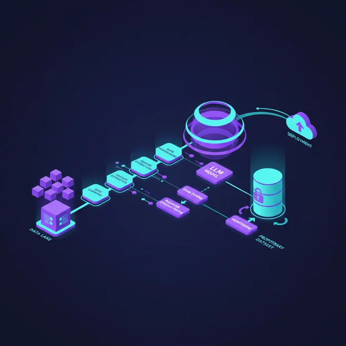

Training an LLM on proprietary data requires selecting the correct adaptation paradigm: parameter-efficient fine-tuning (PEFT/QLoRA) for style and task structure, continued pre-training for massive domain vocabulary ingestion, or retrieval-augmented generation (RAG) for volatile factual recall. Deploying QLoRA on a modern 8B architecture drops the memory threshold from 80 GB of VRAM down to under 16 GB, allowing single-GPU execution without sacrificing task accuracy.
Too many engineering teams push uncurated data straight into full fine-tuning loops, triggering memory out-of-memory (OOM) faults, token degradation, and catastrophic forgetting of foundational reasoning. Adapting an LLM is a systems problem governed by compute budgets, token economics, clean deduplication pipelines, and precise loss telemetry.
This technical blueprint covers the complete architecture: a deterministic decision tree for choosing the right training method, data curation with MinHash locality-sensitive hashing, exact mathematical models for VRAM sizing, and an executable Hugging Face TRL pipeline designed for production clusters.
Architecture Blueprint: Deciding How to Train Your Own LLM
Determining how to train your own llm begins by categorizing the variance between model weights and external facts. Foundation models excel at structural reasoning, linguistic grammar, and broad world knowledge. When engineering systems for proprietary enterprise use cases, you must choose between external context injection and parametric weight adaptation.
The following decision matrix outlines the technical thresholds across corpus volume, latency limits, update cadence, and engineering costs:
| Paradigm | Data Scale | GPU Hardware Required | Update Cadence | Primary Failure Mode |
|---|---|---|---|---|
| Retrieval-Augmented Generation (RAG) | Megabytes to Terabytes | Inference-only (e.g. 1x L4 / A10G) | Real-time / Seconds | Retrieval disconnect, context window truncation |
| LoRA / QLoRA Fine-Tuning | 1,000 to 100,000 instruction pairs | 1x RTX 4090 (24 GB) or 1x A100 (40 GB) | Weekly to Monthly | Catastrophic forgetting, instruction drift |
| Continued Pre-Training | 10 Billion to 100 Billion raw tokens | Multi-node cluster (8x to 64x H100 80 GB) | Quarterly to Bi-annually | Loss divergence, high compute burn |
| Full Pre-Training from Scratch | 1 Trillion+ tokens | Massive cluster (512+ H100s, InfiniBand) | Static release | Underfitting, multimillion-dollar capital drain |
+-------------------------------------------------------------------------+ | DECISION TREE: SELECTING THE CORRECT MODEL ADAPTATION PARADIGM | +-------------------------------------------------------------------------+ | | Is the data frequently updated, volatile, or private per-tenant? | +--- YES ---> [ Implement RAG with Vector DB / Hybrid Search ] | +--- NO | v Does the model need to adopt a custom syntax, schema, or tone? | +--- NO ----> [ Prompt Engineering / In-Context Learning ] | +--- YES | v Is the raw corpus greater than 10 billion unstructured tokens? | +--- YES ---> [ Continued Pre-Training on Unmasked Text ] | | (Then apply LoRA/SFT on downstream tasks) | +--- NO | v [ Parameter-Efficient Fine-Tuning: QLoRA / LoRA via SFT ]Architecture Rule: Never fine-tune solely to inject factual databases that change daily. Use fine-tuning to alter internal behavior, output formatting (such as strict JSON schema conformance), and domain-specific logic. Use RAG to ground the model in real-time, dynamic information.
Pipeline Stage 1: Proprietary LLM Data Collection, Deduplication, and Tokenization
High-performance models require clean datasets. The llm data collection phase demands rigorous ingestion, normalization, and deduplication to prevent model degradation. Feeding boilerplate, duplicated snippets, or noisy HTML dumps directly into training routines degrades cross-entropy loss and encourages memorization over generalization.
- Document Extraction and Parsing: Convert disparate formats (PDFs, Markdown, database dumps, logs) into unified JSON lines (JSONL). Use AST-based parsers for source code and deterministic text parsers to strip markup debris.
- PII Sanitization and Secret Scrubbing: Run regex token matchers and specialized named entity recognition (NER) models to redact API tokens, passwords, Social Security numbers, and personal identity points.
- MinHash LSH Deduplication: Eliminate near-duplicate records. Set a Jaccard similarity threshold (typically 0.75 to 0.85) over 5-gram token shingles to purge repeated content.
- Synthetic Instruction Expansion: Use an enterprise frontier model to generate rich instruction, input, and response triplets from raw text passages.
- Schema Normalization: Format all instruction pairs into standardized ChatML or Alpaca schemas with distinct system, user, and assistant tokens.
The Python script below uses Datasketch to perform MinHash Locality-Sensitive Hashing (LSH) deduplication across raw ingested text records:
import re from datasketch import MinHash, MinHashLSH def extract_shingles(text: str, n: int = 5) -> set: tokens = re.findall(r'\w+', text.lower()) if len(tokens) < n: return {tuple(tokens)} return {tuple(tokens[i:i + n]) for i in range(len(tokens) - n + 1)} def deduplicate_dataset(corpus: list[dict], threshold: float = 0.80, num_perm: int = 128) -> list[dict]: lsh = MinHashLSH(threshold=threshold, num_perm=num_perm) deduplicated_records = [] for idx, entry in enumerate(corpus): text = entry.get("text", "") shingles = extract_shingles(text) m = MinHash(num_perm=num_perm) for s in shingles: m.update(" ".join(s).encode("utf-8")) result = lsh.query(m) if not result: lsh.insert(f"doc_{idx}", m) deduplicated_records.append(entry) return deduplicated_records # Example ingestion run if __name__ == "__main__": raw_data = [ {"id": 1, "text": "PostgreSQL connection timeout occurs when pool reaches capacity."}, {"id": 2, "text": "PostgreSQL connection timeout happens when pool hits total capacity."}, {"id": 3, "text": "Kubernetes ingress controllers route external traffic to pods."} ] unique_data = deduplicate_dataset(raw_data, threshold=0.70) print(f"Retained {len(unique_data)} of {len(raw_data)} records.")Compute Economics: Hardware Sizing and VRAM Calculations for LLM Workloads
Calculating physical memory requirements is critical when deciding how to train llms at scale. An unexpected out-of-memory (OOM) error mid-epoch halts cluster execution and drains compute budgets. Total GPU memory allocation during training includes model parameters, optimizer states, gradients, and activation buffers.
The foundational memory sizing formulas for fine-tuning are defined below:
1. Parameter Memory (M_params):
M_params = P * bytes_per_paramFor 16-bit (BF16/FP16), bytes_per_param = 2. For 4-bit NormalFloat (QLoRA), bytes_per_param = 0.5.
2. Optimizer State Memory (M_opt): Standard AdamW maintains two FP32 states (momentum and variance) plus an FP32 master weight copy for every trainable parameter (P_train):
M_opt = P_train * 16 bytesUnder full fine-tuning, P_train equals the entire model parameter count (P). Under LoRA/QLoRA, P_train is typically between 0.1% and 1.5% of total parameters, drastically cutting optimizer memory.
3. Gradient Memory (M_grad): Gradients store values in 16-bit precision for all trainable parameters:
M_grad = P_train * 2 bytes4. Activation Memory (M_act): Activations scale with sequence length (L), batch size (B), hidden dimension (h), and layer count (n_layers). Enabling activation checkpointing (gradient checkpointing) recomputes intermediate states during the backward pass, reducing activation memory overhead by up to 70% at the cost of approximately 20% more compute cycles.
| Model Size | Training Strategy | Trainable Params | Minimum VRAM | Recommended GPU Architecture |
|---|---|---|---|---|
| 8B (e.g. Llama 3 8B) | Full Fine-Tuning (16-bit) | 8.0 Billion | ~80 GB | 1x H100 (80 GB) or 2x A100 (80 GB, FSDP) |
| 8B (e.g. Llama 3 8B) | LoRA (16-bit base, r=16) | ~20 Million | ~24 GB | 1x RTX 4090 (24 GB) or 1x A10G (24 GB) |
| 8B (e.g. Llama 3 8B) | QLoRA (4-bit base, r=16) | ~20 Million | ~12 to 14 GB | 1x RTX 3060/4070 (16 GB) or 1x T4/L4 |
| 70B (e.g. Llama 3 70B) | Full Fine-Tuning (16-bit) | 70.0 Billion | ~700 GB | 8x H100 (80 GB) via DeepSpeed ZeRO-3 |
| 70B (e.g. Llama 3 70B) | QLoRA (4-bit base, r=32) | ~150 Million | ~48 to 60 GB | 2x A6000 (48 GB) or 1x H100 (80 GB) |
Hardware Sizing Formula: Total VRAM = M_params + M_opt + M_grad + M_act + (1.5 GB CUDA Context Buffer). Always allocate a 20% safety margin above this calculated minimum to absorb dynamic activation spikes during variable-length batch sequences.
Pipeline Stage 2: Executing the LLM Training Process with Hugging Face TRL and QLoRA
Understanding how to train an llm on your own data requires an executable, production-grade training script. In this phase of the llm training process, we combine bitsandbytes 4-bit NormalFloat (NF4) quantization, Hugging Face PEFT for low-rank adaptation, and TRL’s SFTTrainer to run supervised fine-tuning.
This setup injects low-rank adapter matrices into the key attention projections (q_proj, k_proj, v_proj, o_proj) and multilayer perceptrons (gate_proj, up_proj, down_proj). This configuration freezes base model parameters while keeping adapter layers fully trainable.
import torch from datasets import load_dataset from transformers import ( AutoModelForCausalLM, AutoTokenizer, BitsAndBytesConfig, TrainingArguments ) from peft import LoraConfig, get_peft_model, prepare_model_for_kbit_training from trl import SFTTrainer def run_qlora_training(): model_id = "meta-llama/Meta-Llama-3-8B-Instruct" output_dir = "./model-checkpoints/domain-adapted-8b" # Step 1: Configure 4-bit Quantization bnb_config = BitsAndBytesConfig( load_in_4bit=True, bnb_4bit_quant_type="nf4", bnb_4bit_compute_dtype=torch.bfloat16, bnb_4bit_use_double_quant=True ) # Step 2: Initialize Tokenizer & Base Model tokenizer = AutoTokenizer.from_pretrained(model_id, use_fast=True) tokenizer.pad_token = tokenizer.eos_token tokenizer.padding_side = "right" base_model = AutoModelForCausalLM.from_pretrained( model_id, quantization_config=bnb_config, device_map="auto", torch_dtype=torch.bfloat16 ) base_model = prepare_model_for_kbit_training(base_model) # Step 3: Configure LoRA Hyperparameters lora_config = LoraConfig( r=16, lora_alpha=32, target_modules=[ "q_proj", "k_proj", "v_proj", "o_proj", "gate_proj", "up_proj", "down_proj" ], lora_dropout=0.05, bias="none", task_type="CAUSAL_LM" ) model = get_peft_model(base_model, lora_config) model.print_trainable_parameters() # Step 4: Configure Training Hyperparameters training_args = TrainingArguments( output_dir=output_dir, per_device_train_batch_size=2, gradient_accumulation_steps=8, learning_rate=2e-4, lr_scheduler_type="cosine", warmup_ratio=0.03, logging_steps=10, num_train_epochs=3, optim="paged_adamw_8bit", fp16=False, bf16=True, save_strategy="epoch", evaluation_strategy="steps", eval_steps=50, max_grad_norm=0.3, report_to="none" ) dataset = load_dataset("json", data_files={"train": "curated_train.jsonl", "validation": "curated_eval.jsonl"}) trainer = SFTTrainer( model=model, train_dataset=dataset["train"], eval_dataset=dataset["validation"], dataset_text_field="text", max_seq_length=2048, tokenizer=tokenizer, args=training_args ) # Step 5: Execute Training and Persist Adapters trainer.train() trainer.model.save_pretrained(f"{output_dir}/final_adapter") tokenizer.save_pretrained(f"{output_dir}/final_adapter") if __name__ == "__main__": run_qlora_training()Hyperparameter Note: Setting
optim="paged_adamw_8bit"allocates page-locked memory transitions across physical RAM during activation peaks, preventing out-of-memory errors on consumer GPUs with under 24 GB of VRAM.
Production Validation: Benchmarking Loss and Preventing Catastrophic Forgetting
Fine-tuning changes parameter distributions. Teams investigating how to train own llm model instances frequently face catastrophic forgetting, where the model masters domain terminology but loses foundational logical deduction, code synthesis, or instruction adherence. Validating your model requires a dual-track strategy: quantitative loss tracking and qualitative LLM-as-a-judge benchmarking.
To prevent catastrophic forgetting, construct an anchor replay buffer. Mix between 10% and 20% of general-domain instruction pairs (such as OpenHermes or SlimPajama samples) into your proprietary training dataset. This keeps activation paths through core reasoning sub-networks stable during backpropagation.
import json from openai import OpenAI def llm_judge_evaluation(prompt: str, ground_truth: str, generated_output: str) -> dict: client = OpenAI(api_key="your-api-key") judge_system_prompt = """ You are an impartial, highly rigorous systems engineer. Evaluate the candidate response against the reference ground truth across three dimensions: 1. Factual Accuracy (0-5) 2. Adherence to Technical Schema (0-5) 3. Hallucination Penalties (0-5, where 5 is zero hallucinations) Provide output in strict JSON format matching the schema: {"accuracy": int, "schema": int, "hallucination": int, "reasoning": str} """ user_payload = f"Prompt: {prompt}\nReference: {ground_truth}\nCandidate: {generated_output}" response = client.chat.completions.create( model="gpt-4o", response_format={"type": "json_object"}, messages=[ {"role": "system", "content": judge_system_prompt}, {"role": "user", "content": user_payload} ], temperature=0.0 ) return json.loads(response.choices[0].message.content)Track the following production validation checklist before merging adapter weights into runtime inference servers:
- Loss Divergence Check: Ensure validation loss consistently tracks training loss. If validation loss curves upward while training loss plunges past epoch 2, stop training immediately to prevent overfitting.
- Perplexity Boundary: Measure perplexity on a held-out domain test set. Expect steady reductions without irregular spikes across standard sequence boundaries.
- Replay Buffer Calibration: Benchmark against standard MMLU or GSM8K subsets to verify that zero-shot logic retains at least 95% of the base model baseline score.
- Latency Profiling: Verify that merged model weights (combining base FP16 with LoRA adapters) load and serve via vLLM or TensorRT-LLM without runtime inference regression.
Frequently Asked Questions
When should you fine-tune an LLM instead of using RAG?
Use RAG when injecting dynamic, rapidly changing factual knowledge without modifying model behavior. Fine-tune on your own data when the model must adopt specialized terminology, output structured formats reliably, or internalize complex domain-specific reasoning that system prompts cannot achieve.
What hardware is required for the LLM training process using QLoRA?
Training an 8B parameter model using QLoRA requires a single GPU with at least 16GB to 24GB VRAM, such as an NVIDIA RTX 4090 or A10G. Full 16-bit fine-tuning of the same model requires roughly 64GB to 80GB VRAM (A100 or H100).
What is the primary risk during the llm data collection phase?
The primary risk during collection is contamination from duplicated text, unmasked PII, and poor formatting quality. Low-quality tokens degrade training loss, trigger memorization anomalies, and cause the model to hallucinate incorrect domain patterns.
How can teams avoid catastrophic forgetting when learning how to train own LLM model weights?
Mitigate catastrophic forgetting by mixing 10 to 20 percent general instruction data into your domain dataset as an anchor replay buffer. Additionally, keep LoRA rank (r) conservative and use a lower learning rate with cosine decay.
Training an LLM on your own data moves model performance from generic completions to deterministic, domain-native system execution. By taking a structured engineering approach (filtering datasets with MinHash LSH, sizing memory allocations mathematically, and using QLoRA with paged optimizers), you can train high-accuracy 8B and 70B models on accessible GPU hardware.
Once training completes, merge adapter weights directly into the base model checkpoints or mount them as dynamic runtime adapters using inference runtimes like vLLM or TensorRT-LLM. Continuously validate checkpoints against an automated evaluation pipeline to maintain performance and eliminate regressions in production.